Dissecting Relu: A desceptively simple activation function

What is this post about?

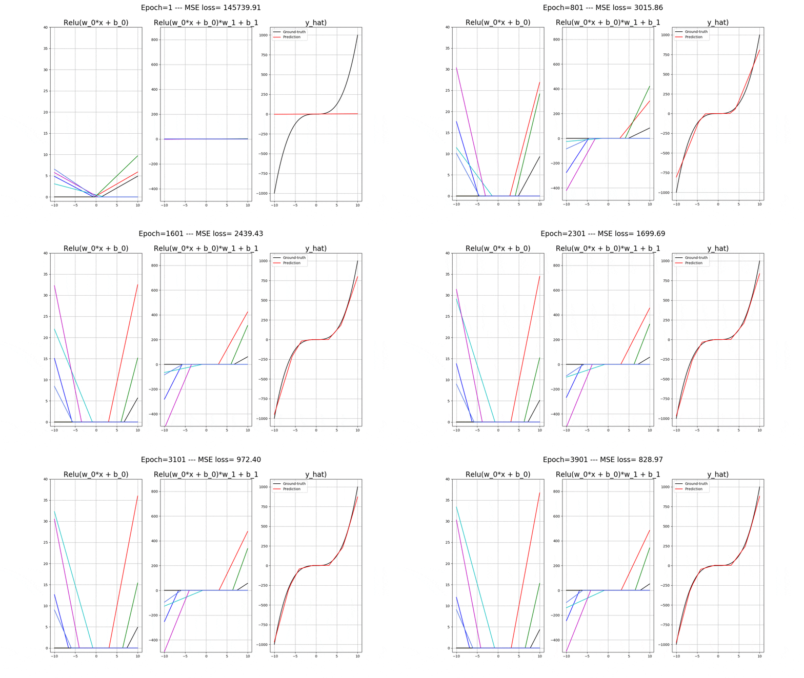
This is what you will be able to generate and understand by the end of this post. This is the evolution of a shallow Artificial Neural Network (ANN) with relu() activation functions while training. The goal is to fit the black curve, which means that the ANN is a regressor! The full code for this entire post is available on MLDawn’s GitHub.

Relu is a desceptively simple Activation Function that is commonly used to introduce non-linearity into Artificial Neural Networks. Funny enough, this simple function can do a ton of cool stuff. In this post, we will understand the flexibility of Relu, its derivation, as well as, its derivative. We will also, write up some code to see the evolution of a collection of Relu functions, second by second, as they strive to fit curves. In this post you will learn the following:

What is Relu and why is it good? What are the mathematical properties of Relu and how this seemingly inflexible function can give us a high degree of non-linearity?
How to write up a simple Artificial Neural Network in Python and PyTorch with Relu activation functions, and fit interesting curves, hence the non-linearity!
You will also learn how to observe the evolution of these Relu functions during training and generate an animation of it.

I am ready when you are 😉

What is Relu?

We have previously discussed Artificial Neural Networks (ANNs) and even gone through the details of Gradient Descent (Part-1 and Part-2 are available). Today it is time to dive more into the details of ANNs and study one of the most common activation functions ever invented, that is Relu.

Relu stands for Rectified Linear Unit and it is a popular activation function that is used in ANNs prevalently. It has certain advantages that its predecessors, Sigmoid (used during the early 1990s) and Tanh (used later in 1990s and through the 2000s), lack.

For instance, both Sigmoid and Tanh suffer from the saturation problem as the gradient value near either of the extremes of these 2 functions approaches 0! This means that during training an ANN, while doing back-propagation, we will suffer from infinitesimal gradient values (effectively 0’s) and this means that training will slow down! This is called the vanishing gradient problem.

… sigmoidal units saturate across most of their domain—they saturate to a high value when z (i.e., their input) is very positive, saturate to a low value when z is very negative, and are only strongly sensitive to their input when z is near 0. — Page 195, Deep Learning, 2016

As noted above, the other issue with both Sigmoid and Tanh is that they both are sensitive to changes only near their mid-point and as you go to either of the extremes of these 2 functions, their sensitivity lessens, which is where their gradient approaches 0. It is only near their mid-point that they have a nice non-linear behavior, but they approach a linear behavior as you go farther away from their mid-points.

Mathematically speaking, Relu(z) can be defined as follow:

$relu(z) = max(0, z)$

Coding and Visualizing

We can plot it to have a better visual understanding of it. Let’s use Python and matplotlib to do this. First, let’s import the necessary packages:

import numpy as np
import matplotlib.pyplot as plt

And now let’s define the relu(z) function in Python:

def relu(z):
    if z > 0:
        return z
    else:
        return 0

Now let’s plot relu(). This code will do it:

# Define linewidth and fontsize to control the aesthetics of the plots easily
linewidth = 4
fontsize = 20

# Define a range of values for the inputs of relu(z)
z_range = np.arange(-5,5, 0.01)

plt.figure(figsize=(16,9))
# For each z in x_range compute relu(z)
y_relu = [relu(z) for z in z_range]
plt.plot(z_range, y_relu, c='b', linewidth= linewidth, label='Relu(z)')
plt.ylim(-5, 5)
plt.xlim(-5, 5)
plt.grid()
plt.legend(fontsize=fontsize, loc=2)
plt.show()

Whose output is the mighty relu function:

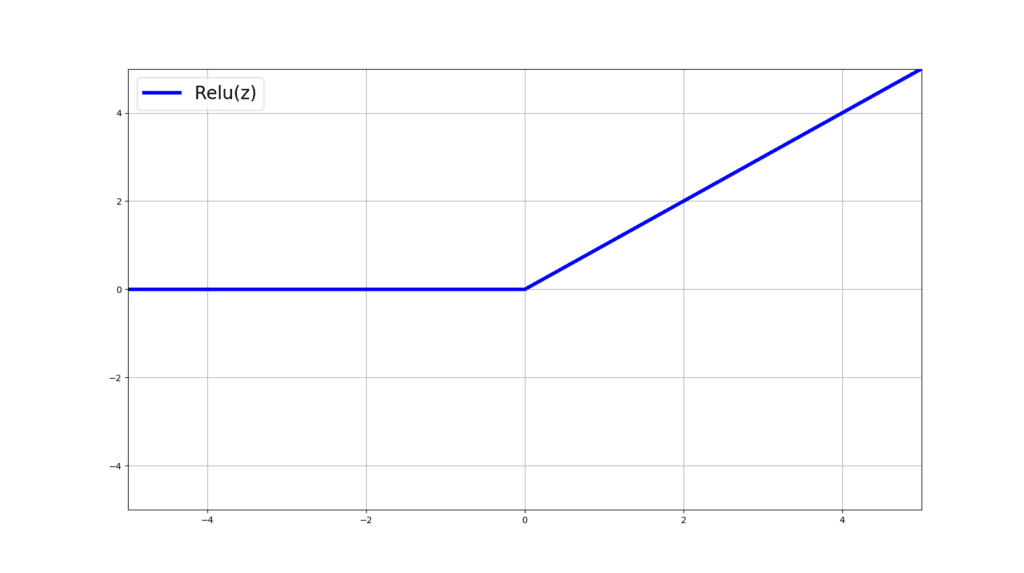
I agree! It seems far less fancy than Sigmoid or Tanh but believe me, this desceptively simple function has a lot to offer and is far more flexible than it looks. In the next section we will understand the derivative of relu.

Understanding the Derivative of Relu

As you may have noticed, relu(z) is differentiable in all of its domain except when z=0. In other words, the left and right derivatives at z=0 exist BUT are not equal (i.e., at z=0, relu(z) is not differentiable). Then how is that it can be used in gradient-based learning methods such as in Artificial Neural Networks (ANNs)? During computing the gradients, what happens if we hit z=0? Would gradient descent and back-propagation simply fail?

The derivalive of relue(z) can be studied in 3 regions of its domin, namely, when z>0, z<0, and z=0. Let’s see the value of the gradients for the first two cases first:

$\frac{\partial relu(z)}{\partial z} = \begin{cases} 0 & \quad \quad z<0 \\\\\\\\\\\\\\\\\\\\ 1 & \quad \quad z>0 \end{cases}$

This is easy to follow, right? Well, for all positive values of z, the slope of the tangent line is going to be 1. Similarly, for all z<0, this slope is 0. Now what about when z=0? Well relu(z) is not differentiable at z=0:

The left derivative of relu(z) w.r.t z is 0 and the right derivative is 1. However, since they are not equal, then relu(z) at z=0 does not exist! This effectively means that, the rate of change of relu(z) w.r.t z, at z=0, is different depending on whether you are getting infitely close to z=0 from its left side, or its right side (take a moment to absorbe this 😉 if that doesn’t make sense).

So, whet do we do? We do know that if we use relu(z) in training an ANN, we need to make sure that we can compute its derivative for all possible values of z! Here are a few ways to think about this problem:

In an Artificial Neural Network (ANN), for a given neuron with relu(z) activation function, the chances of the pre-activation value z becoming exactly 0 is infinitesimally low!
If by some unfortunate and unlikely disaster z becomes equal to exactly 0, then you might be tempted to just pass a random value as the gradient of relu(z) w.r.t z at z=0. Interestingly, since z=0 is a rare event, even with a random value for the gradient, the optimization process (e.g., gradeint descent) would get barely affected! It is like you update the parameters of your neural network towards a wrong direction once in a blue moon. Big deal!
In certain platforms of deep learning such as Tensorflow, when z=0, the derivative of relu(z) w.r.t z is computed as 0. Their justification is that we should favour more sparce outputs for a better training experience.
Some would choose the exact value of 0.5 as the gradient of relu(z) w.r.t z at z=0. Why? Well they argue that since the left and right gradients of relu(z) at z=0 are either 0 and 1, it makes sense to choose the mid-point 0.5 as the value of the gradient of relu(z) at z=0. This does not make much sense to me, personally!

Using Sub-Gradients

I don’t like thinking about the gradient of relu(z) at z=0 as just a random and arbitraty value. Let’s use the idea of sub-gradients and plot infinite number of lines, touching relu(z) at z=0! Effectively, we will have infinite number of slopes ranging from 0 all the way to 1, since we start from a horizontal line with a slope of 0 and end up with the final line which will land on relu(z) itself, and will have a slope of 1. You can think of g as a uniform random variable representing the slopes of these lines:

These slopes are called the sub-gradients of relu(z) at z=0.

The way, I personally, would choose a candidate value out of all of these slopes as the gradient of relu(z) at z=0, is by taking the expectation of the random variable g (i.e., what we expect the gradient of relu(z) at z=0 be using these sub-gradients). Remember that g is uniformly distributed! So, visually speaking, this is what I mean:

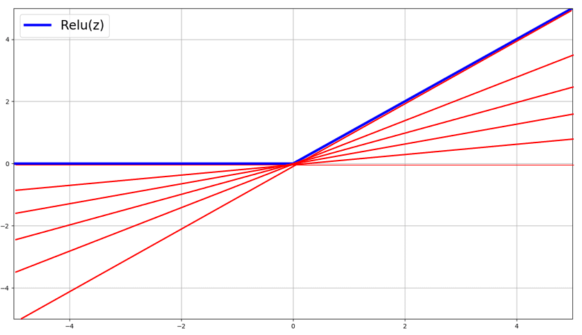
The slopes of these red lines, g, are the sub-gradients of relu(z) at z=0, where g is uniformly distributed! We know that for a given random variable g, with a certain probability distribution p(g) in the interval [a,b] the expectation is equal to:

$E(g) = \int_{a}^{b} {g \times p(g) dg}$

And when g is uniformly distributed in the interval [a, b], p(g) must be:

$p(g) = \frac{1}{b-a}$

So that the area under the curve would be exactly equal to 1. More specifically, this is a rectangular area, whose length is equal to $(b-a)$ and whose width is $\frac{1}{b-a}$ . And clearly, the area of this rectangel is 1:

$\int_{a}^{b} {p(g) dg}=(b-a) \times \frac{1}{(b-a)}=1$

Otherwise, p(g) cannot be a probability distribution! In our case, the range [a,b] is equal to [0,1], as this is the range of possible values for the slopes of these sub-gradients.

Now, back to computing the expectation of these bloody sub-gradients (i.e., slopes of infite number of those red lines at z=0) represented by g:

$\int_{a}^{b} {g \times p(g) dg} = \int_{a}^{b} {g \times \frac{1}{(b-a)} dg}$

From there let’s replace [a,b] with [0,1]:

$\int_{0}^{1} {g \times dg}$

So:

$E(g) = \int_{0}^{1} {g \times dg} = \frac{g^2}{2} \qquad \qquad |^{1}_{0} = \frac{1}{2} - \frac{0}{2}= 0.5$

So, the expected value of the sub-gradient over infinitie number of sub-gradients is 0.5! I know! We ended up with the mid-point in the range [0,1]. However, I am more convinced by the “Expectation” arguement than I am with the “mid-point” arguement. So, this means that when z=0 (as rare as it is), define the candidate sub-gradient to be:

$\frac{\partial relu(z)}{\partial z} = E(g) = 0.5$

Moral of the story: You can choose any value in the range [0,1] and your ANN will still train. However, I like my expectation arguement as it lays a consistent arguement rather than just picking a random value!

The Flexibility of Relu(z)

ANNs manipulate relu(z) during their training in all sorts of way. Let’s see how flexible can relu(z) get, given simple mathematical manipulations. By simple manipulations of relu(z), you can flip, rotate, or shift the relu(z) function:

# define a range for the pre-activations
z_range = np.arange(-5,5, 0.01)

plt.figure(figsize=(16,9))
plt.suptitle('The Flexibility of Relu(z)', fontsize=fontsize)

plt.subplot(2,2,1)
y_relu = [relu(z) for z in z_range]
plt.plot(z_range, y_relu, c='b', linewidth= linewidth, label='Relu(z)')
plt.ylim(-5,5)
plt.xlim(-5,5)
plt.grid()
plt.legend(fontsize=fontsize, loc=2)

plt.subplot(2,2,2)
y_relu = [relu(-z) for z in z_range]
plt.plot(z_range, y_relu, c='k', linewidth= linewidth,label='Relu(-z)')
plt.ylim(-5,5)
plt.xlim(-5,5)
plt.legend(fontsize=fontsize,loc=1)
plt.grid()

plt.subplot(2,2,3)
y_relu = [-relu(z) for z in z_range]
plt.plot(z_range, y_relu, c='r', linewidth= linewidth,label='-Relu(z)')
plt.ylim(-5,5)
plt.xlim(-5,5)
plt.legend(fontsize=fontsize,loc=2)
plt.grid()

plt.subplot(2,2,4)
y_relu = [-relu(-z) for z in z_range]
plt.plot(z_range, y_relu, c='g', linewidth= linewidth,label='-Relu(-z)')
plt.ylim(-5,5)
plt.xlim(-5,5)
plt.legend(fontsize=fontsize,loc=1)
plt.grid()

plt.show()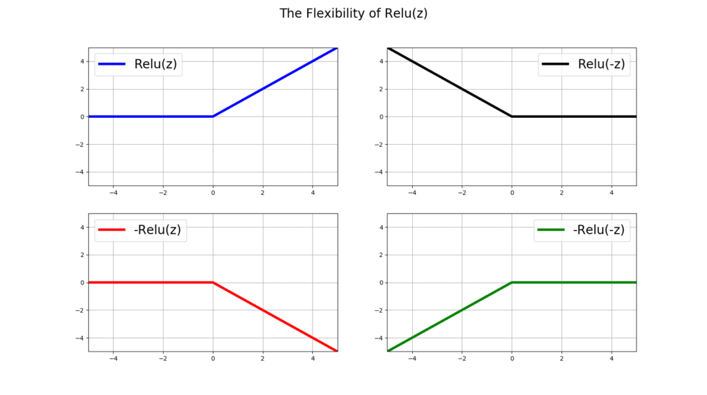

You can also change the slope of relu(z), by multiplying z by a weight w:

# Define a range for some values for the coefficient w
w_range = np.arange(0.5, 3.5, 0.5)
plt.figure(figsize=(16, 9))
plt.suptitle('Changing the slope of Relu(w*z) using a coefficient w', fontsize=fontsize)
for idx, w in enumerate(w_range):
    plt.subplot(2,3,idx+1)
    y_relu = [relu(w*z) for z in z_range]
    plt.plot(z_range, y_relu, c='b', linewidth=linewidth, label='w = %.2f' % w)
    plt.ylim(-1, 5)
    plt.xlim(-5, 5)
    plt.grid()
    plt.legend(fontsize=fontsize, loc=2)
plt.show()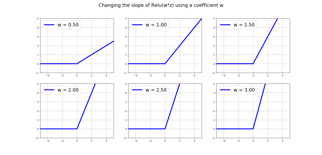

Hell you can even move the bloody thing horizentally using a bias term b in the form of relu(z + b):

# Define a range for some values for the coefficient w
w_range = np.arange(0.5, 3.5, 0.5)
plt.figure(figsize=(16, 9))
plt.suptitle('Changing the slope of Relu(w*z) using a coefficient w', fontsize=fontsize)
for idx, w in enumerate(w_range):
    plt.subplot(2,3,idx+1)
    y_relu = [relu(w*z) for z in z_range]
    plt.plot(z_range, y_relu, c='b', linewidth=linewidth, label='w = %.2f' % w)
    plt.ylim(-1, 5)
    plt.xlim(-5, 5)
    plt.grid()
    plt.legend(fontsize=fontsize, loc=2)
plt.show()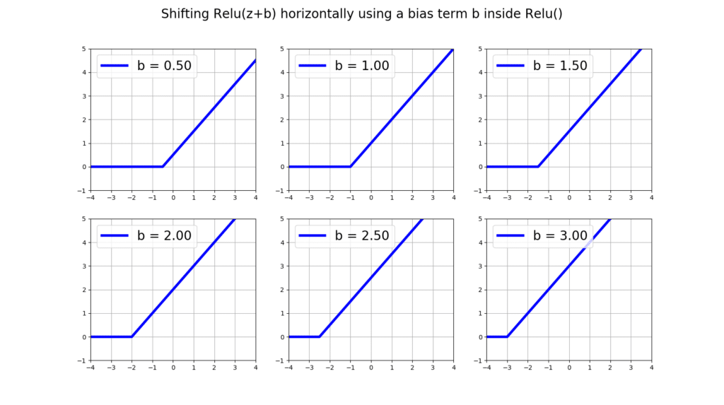

Or vertically using a bias term ourside relu(z) in the form of relu(z) + b:

bias = np.arange(0.5, 3.5, 0.5)
plt.figure(figsize=(16, 9))
plt.suptitle('Shifting Relu(z) + b vertically using a bias term b outside Relu()', fontsize=fontsize)
for idx, b in enumerate(bias):
    plt.subplot(2,3, idx+1)
    y_relu = [relu(z)+b for z in z_range]
    plt.plot(z_range, y_relu, c='b', linewidth=linewidth, label='b = %.2f' % b)
    plt.ylim(-1, 5)
    plt.xlim(-4, 4)
    plt.grid()
    plt.legend(fontsize=fontsize, loc=2)
plt.show()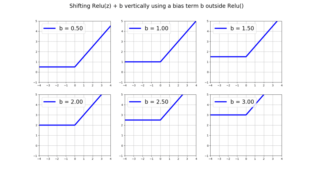

Now, let’s see how an Artificial Neural Network (ANN) can use all of this flexibility to give us the non-linearity that relu() has been boasting about all these years.

Training an Artificial Neural Network with Relu() Fctivation Functions to fit a Curve

Let’s onsider a 1-layer ANN with 1 input and 1 output. Essentially, we will us it for the task of regression where given the input we will predict a real-valued output. The activation functions in the hidden layer are all relu(), and we have 2 bias units, one for the hidden layer and one for the output layer. Let’s denote all of the weights connecting the input data to the hidden layer with $w_0$ and all of the bias weights connecting to the hidden layer with $b_0$ . Simiarly, let’s call all the weights conecting the hidden layer to the output node as $w_1$ and the bias unit connectting to to the output node with $b_1$ .

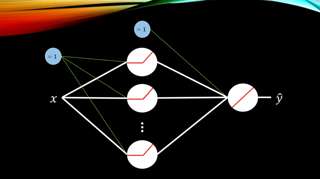
So, let’s get comfortable with the math. The activations at the hidden layer for each relu() is:

$Relu(w_0 \times x + b_0)$

The final output of the model is then (Remember: The output neuron has a purely LINEAR activation function):

$\hat{y} = Relu(w_0\times x + b_0)\times w_1 + b_1$

Now let’s code up a regressor using Pytorch, which can receive a desirable number of relu() neurons in its hidden layer, as an arguement. But first, let’s look at the curve that we would like the ANN learn to fit:

plt.figure(figsize=(16, 9))
x = torch.unsqueeze(torch.linspace(-10, 10, 300), dim=1)
y = x.pow(3)
plt.plot(x.data.numpy(), y.data.numpy(), color="k", label='Ground-truth')
plt.legend(fontsize=fontsize,loc=2)
plt.grid()
plt.show()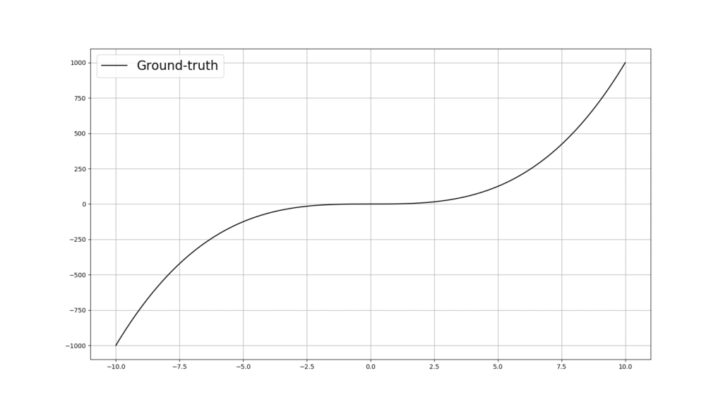

Now, let’s define the device on which we would like to put our data and our ANN model. This can be either the CPU or the GPU. This code, will try to assign GPU as our device, if not posible, then inevitably we are stuck with the CPU:

use_gpu = torch.cuda.is_available()
# If so, change torch.device to 'gpu'
device = torch.device("cuda" if use_gpu else "cpu")

Let’s build our regressor:

class Regressor(nn.Module):
    def __init__(self, n_hidden=2): # n_hidden is 2 by default but can 
        #be passed as an arguement
        super(Regressor, self).__init__() # Accessing he __init__ constructor in nn.Module
        self.hidden = torch.nn.Linear(1, n_hidden)  # hidden layer
        self.predict = torch.nn.Linear(n_hidden, 1)  # output layer with only 1 neuron

    def forward(self, x):
        x = F.relu(self.hidden(x)) # Applying relu()
        x = self.predict(x) # Gnerating y_hat
        return x

Now let’s create an object of the regressor class and setup some initial stuff for the training to take place:

# number of relu() units
n_hidden = 7
# total number of epochs
n_epochs = 4000
# Building an object from the regressor class while  passing
# n_hidden and setting the model to train() mode
regressor = Regressor(n_hidden=n_hidden).train()
# Defining the optimizer
optimizer = torch.optim.SGD(regressor.parameters(), lr=0.0001)
# Defining MSE as the appropriate los function
# For regression.
loss_func = torch.nn.MSELoss()

Now let’ start the training:

plt.figure(figsize=(16, 9))
for epoch in range(n_epochs):
    # Put the model in training mode
    regressor.train()
    # This is there to clear the previous plot in the animation
    # After each epoch
    plt.clf()
    # input x to the regressor and receive the predicion
    y_hat = regressor(x)
    # Compute the loss between y_hat and the actual
    # Value of the ground-truth curve, y
    loss = loss_func(y_hat, y)
    # Compute the gradients w.r.t all the parameters
    loss.backward()
    # Update the parameters
    optimizer.step()
    # Zero out all the gradients before inputing the next data point
    # Into the regressor model
    optimizer.zero_grad()

    # Every 100 epoch evaluate do some plotting
    if epoch % 100 == 0:
        print('Epoch %d --- Loss %.5f' % (epoch+1, loss.data.numpy()))
        # Bbefore evaluation, put the model back to evaluation mode
        regressor.eval()
        # At this very moment of training, grab the current biases and weights
        # From the model object, namely, b_0, b_1, w_0, and w_1
        biases_0 = regressor.hidden.bias.cpu().detach().numpy()
        weights_0 = regressor.hidden.weight.squeeze(0).cpu().detach().numpy()
        biases_1 = regressor.predict.bias.cpu().detach().numpy() # This has ONLY 1 value
        weights_1 = regressor.predict.weight.squeeze(0).cpu().detach().numpy()

        # For the purpose of plotting consider the current range of
        # x as the inputs to EACH relu() individualy
        data = x.detach().numpy()
        # This will hold the UNLIMATE
        # prediction, that is, relu(input*w_0+b_0)*w_1 + b_1
        # We reset it before plotting the current status of the model
        # And the learned relu() functions
        sum_y_relu = []
        # For each relu() unit do the following
        for idx in range(n_hidden):

            plt.suptitle('Epoch=%d --- MSE loss= %.2f' % (epoch+1, loss.data.numpy()), fontsize=fontsize)
            # Plot output of the current relu() unit
            plt.subplot(1,3,1)
            plt.title('Relu(w_0*x + b_0)', fontsize=fontsize)
            y_relu = [relu(d*weights_0[idx]+biases_0[idx]) for d in data]
            plt.plot(data, y_relu)
            plt.ylim(-1,40)
            plt.grid()

            plt.subplot(1, 3, 2)
            # Plot output of the current relu(), multiplied by its
            # corresponding weight, w_1, and summed with the bias b_1
            plt.title('Relu(w_0*x + b_0)*w_1 + b_1',fontsize=fontsize)
            y_relu = [relu(d*weights_0[idx]+biases_0[idx])*weights_1[idx] + biases_1[0] for d in data]
            plt.plot(data,y_relu)
            plt.ylim(-500,900)
            plt.grid()

            # Kee adding the Relu(w_0*x + b_0)*w_1 + b_1 for each relu to the
            # sum_y_relu list. We will sum them up later to plot
            # The ULTIMATE predction of the model y_hat
            sum_y_relu.append([relu(d*weights_0[idx]+biases_0[idx])*weights_1[idx] + biases_1[0] for d in data])

        # Sum it all up
        sum_y_relu = np.sum(np.array(sum_y_relu),axis=0)
        plt.subplot(1, 3, 3)
        plt.title('y_hat)', fontsize=fontsize)
        plt.plot(x.data.numpy(), y.data.numpy(), color="k", label='Ground-truth')
        plt.plot(data,sum_y_relu, c='r', label='Prediction')
        plt.legend()
        plt.grid()

        # A slight delay in the animation
        plt.pause(0.1)

The following animation will pop out, where you can nicely track the evolution of these amazing relu()’s:

Conclusion

Appearances can be desceptive! Relu() is a very strong activation function which can bring us non-liniarity, and it does not have the issues that its predecesors, Sigmoid() and tanh() had. Namely with relu you can enjoy its properties: 1) No saturation 2) No vanishing gradient 3) Non-liniarity.

On behalf of MLDawn, Mind yourself 😉